How to power customer acquisition marketing campaings?
Udacity Data Scientist Nanodegree Capstone Project
Acquiring new customers is a challenge most businesses have faced, are facing or will still face. It’s a delicate task and it envolves getting to know your existing customers to better understand their behaviour and therefore, be able to focus on attracting more individuals like them!
So that’s what we’ll be doing here. This project’s goal is to predict which individuals are most likely to convert into becoming customers for a company in Germany (Arvato Financial Solutions).
This is done based on an analysis of the demographics data for customers compared to demographics data for the general population of Germany.
Unsupervised learning techniques were used to perform customer segmentation and identify the parts of the population that best describe the core customer base of the company.
After that, a classification model was built to make predictions such as which individuals are most likely to respond to a marketing campaingn and become customers for the company.
The data used was provided by Bertelsmann Arvato Analytics, and represents a real-life data science task.
Project steps
This project is composed of the following steps:
- Data Preparation: preparation of the data provided.
- Customer Segmentation: attribute analysis of established customers and the general population in order to create customers segments and be able to identify people of interest within the population.
- Classification Model: the previous analysis will be used to predict what individuals will respond to the marketing campaing so that the company can focus on them instead of the entire population. PyCaret library will be used for this task!
Step 1: Data Preparation
Data Sampling
The code for this part can be accessed here.
The datasets provided for this projects are too large. To avoid problems as we develop the project, I’ve decided to take a sample of both datasets to work with. A random sampling of 25% of the datasets with no replacing was done.
Rows of full AZDIAS dataset:      891221
Rows of sample AZDIAS dataset:    222805

Rows of full CUSTOMERS dataset:   191652
Rows of sample CUSTOMERS dataset:  47913
Data Cleaning
The code for this part can be accessed here.
A few cleaning functions were needed in order to get all the job done, so here’s a summary of all the cleaning steps:
- replaced wrong values of entries (‘X’ and ‘XX’ entries were found in some columns);
- replaced NaNs with -1 in determined columns where -1 means the value is unknown;
- dropped columns for having over 40% of null values;
- imputted fixed values to columns where the fixed value means unknown;
- imputted the most frequent value to the remaining columns (because it’s categorical columns, it makes sense to imput the most frequent and not the mean or the median, for exemple, as that would imput a non existing value to the category);
- replaced values of columns according to the attributes meaning and description files;
- replaced string and wrong values in binary categorical columns.
After all the cleaning steps, I made a feature selection based on correlation (dropped columns with over 85% correlation coefficient) and attribute meaning.
Feature engineering was also done in a column that had too many categories. It was divided in two columns according to the meaning of each category.
At the end of this step, I made sure the columns dtypes were correct.
AZDIAS:      (222805, 366)
CUSTOMERS:    (47913, 369)
TRAIN:        (42962, 367)
TEST:         (42833, 366)Final AZDIAS:     (222805, 309)
Final CUSTOMERS:   (47913, 309)
Final TRAIN:       (42962, 310)
Final TEST:        (42833, 309)
Step 2: Customer Segmentation
The code for this part can be accessed here and here.
Finally we have clean data to get started with the unsupervised learning model!
KModes model is the one we chose because our variables are categorical.
KMeans (most commonly used clustering algorithm) uses distance to cluster data (the lesser the distance, the more similar the data points are so they are more likely to get clustered together). It makes a lot of sense to use it for continuous data.
But in this case, as we are dealing with categorical data points, it doesn’t make sense to use distance measures. KModes uses the dissimilarities, which means how mismatching the data points are between each other. The lesser the dissimilarities, the more similar the data points are so they will be clustered together.
As KMeans uses means, KModes uses modes instead.
Let’s get started! Firstly, I run some experiments regarding preprocessing for modeling (the code for this part can be accessed here).
Approach 1 — No preprocessing
I ran the KModes method for a range 2 to 10 clusters with no preprocessing (like scaling, etc.) done to the data.
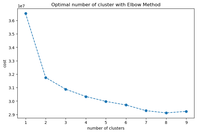
Although we have a clear elbow on 2 clusters, it doesn’t seem like a good number to adopt in this situation. In order to identify patterns on the population that would help identify new potential customers, we need to have more groups than just 2.
So let’s test another approach and see if we get different results.
Approach 2 — Data Scaling and PCA
Now I scaled the data with StandardScaler.
After that, I ran a PCA method (to reduce the dimentionality) for every two components on the dataset so I could see how the explained variance ration would vary.
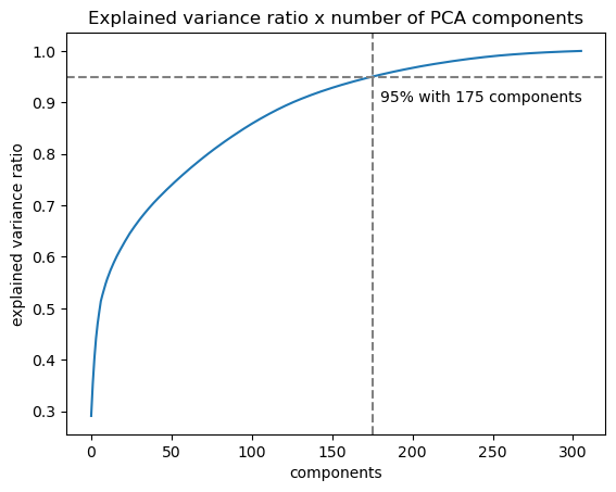
As shown on the plot above, I picked 175 components that gives me a 95% variance explainability.
With the scaling and dimensionality reduced, I then ran the KModes method again for the same range.
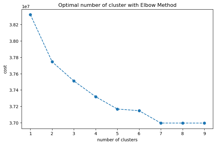
In this new approach, we have a more realistic plot, but the cost went up.
In this case, we’ll use n=5 for clustering without any previous preprocessing steps.
Modeling
Now it’s time to start the modeling phase!
As we’ve already tested a couple approaches on the previous notebook, now it’s time to implement the chosen model.
I’ve chose to use k=5 clusters because it showed an interesting cost value (the sum of all the dissimilarities between the clusters) after the observed elbow on k=2.
# Convert dataframes to matrix
azdiasMatrix = azdias.to_numpy()
customersMatrix = customers.to_numpy()k = 5
kmodes = KModes(n_clusters = k, init = 'Huang', random_state = random_state)# train model and make predictions
y_pred_azdias = kmodes.fit_predict(azdiasMatrix)
y_pred_customers = kmodes.predict(customersMatrix)# create cluster column and add to the dataframes
azdias['cluster'] = kmodes.labels_
customers['cluster'] = y_pred_customers
Evaluating
The elbow method is used to determine the k for KModes and it's also an evaluating metric.
Interpreting the results
Now that we’ve got our clusters in the datasets, let’s create a new dataset with the amount of indivuduals in each cluster for each of the datasets. This way we can make some plots to better visualize how they’re distributed.
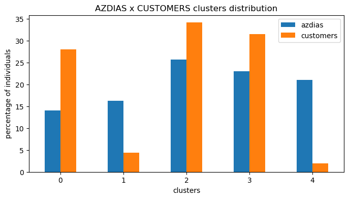
Now we’re talking!! Look at how significant that simple plot can be.
We can see clearly that clusters 0, 2 and 3 are a strong representation of our customers compared to the population.
Clusters 1 and 4 are the ones with less representativity of our customers.
With that in mind, let’s get down to getting to know those clusters that best represent our customers so we can draw sort of a profile of them.
# columns for centroids
cluster_col = ['cluster']
cols = [col for col in azdias if col not in cluster_col]# make index for cluster interpretation
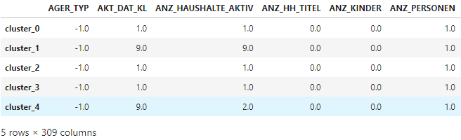
index = ['cluster_0', 'cluster_1', 'cluster_2', 'cluster_3', 'cluster_4']# make dataframe
df_clusters_centroids = pd.DataFrame(kmodes.cluster_centroids_, columns = cols, index = index)
df_clusters_centroids
azdias_centroids = df_clusters_centroids.loc[(df_clusters_centroids.index == 'cluster_1') | (df_clusters_centroids.index == 'cluster_4')]
customers_centroids = df_clusters_centroids.loc[(df_clusters_centroids.index == 'cluster_0') | (df_clusters_centroids.index == 'cluster_2') | (df_clusters_centroids.index == 'cluster_3')]centr_dict = {'population': list(azdias_centroids.mean()),
              'customers': list(customers_centroids.mean())}df_centr = pd.DataFrame(centr_dict, columns = ['population', 'customers'], index = df_clusters_centroids.columns)
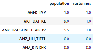
From those two datasets created above, we can see the demographic points for the centroids of each cluster, that way, if we examine each column we can see what kind of individuals are on clusters 0, 2 and 3 (most likely customers) and on clusters 1 and 4 (most likely not out customers).
Step 3: Classification model
The code for this part can be accessed here.
Now it’s time to build a model to predict which individuals are worth targeting on the marketing campaing to acquire more customers.
Let’s check how the target variable is balanced on the dataset.
0    42430
1      532
Name: RESPONSE, dtype: int64


Response = 1.25 %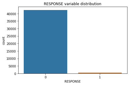
As we can see from the plot, we’ve got a HIGHLY INBALANCED dataset on the target variable.
This will certainly be a challenge for our task!
Metrics Selection
Before we get our hands on modeling, let’s determine which metrics we’ll be using to evaluate the model afterwards.
It’s important to have this step previously to building the model so we don’t get biased by the results.
Accuracy:
For this task, with a highly imbalanced dataset as we’ve stated, it definitelly doesn’t make sense to use accuracy to evaluate our model. The accuracy score is the fraction of correct predictions. In imbalanced datasets, accuracy will be close to 100% even if we were to predict all data points to 0 (dummy classifier).
Precision, Recall and F-measures:
TP (true positives) - Positive predicted as positive (correct prediction)
TN (true negatives) - Negative predicted as negative (correct prediction)
FN (false negatives) - Positive predicted as negative (incorrect prediction)
FP (false positives) - Negative predicted as positive (incorrect prediction)Precision: out of all positive predictions (TP + FP), how many were predicted correctly (TP)?
TP / (TP + FP)Recall: out of all actual positive samples (TP + FN), how many were predicted correctly (TP)?
TP / (TP + FN)F1 Score is the harmonic mean of precision and recall, so it’s a good metric to evaluate a model like ours.
Area Under the ROC curve (AUC):
The ROC (Receiver operating characteristic) curve is a plot of the true positive rate (TPR = fraction of TP out of the positives or sensitivity) vs. the false positive rate (FPR = fraction of false positives out of the negatives or specificity) as the threshold varies.
So the closer to 1 the area under the ROC curve is, the closer the sensitivity and specificity are to the sweet spot.
In this case, we want to keep a close eye for F1 score and also AUC score.
Modeling
We’ll use pycaret to run several models so we can choose from.
The setup function initializes the training environment and creates the transformation pipeline. It takes two mandatory parameters: data and target. And preprocessing parameters are optional.
As preprocessing parameters, here’s what we’ll adopt:
- normalization of data with z-score: the mean is 0 and the standard deviation is 1
- balancing of target variable with Synthetic Minority Oversampling Technique, or
SMOTEmethod: it creates synthetic examples for the minority class.
When the setup is executed, pycaret takes care of data types inferation for all features based on certain properties. After that, it displays a prompt asking for data types confirmation (this step can’t be seen on an already ran cell).
# setting up pycaret with normalization and balancing
s = setup(df_train, target = 'RESPONSE',
          normalize = True,
          fix_imbalance = True)
The compare_models is where the training happens. It trains and evaluates the performance of all the estimators available in the model library using cross-validation.
It outputs a scoring grid with the average cross-validated scores for each trained model. The grid by default is sorted using ‘Accuracy’ so we’ll change it to sort by ‘auc’ instead (metric we previously decided to use).
# run models to compare
best = compare_models(sort = 'auc')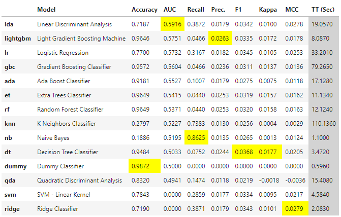
As I had said before, the accuracy is very high for the dummy classifier, as well as for several other models because of how imbalanced the dataset is on the target feature.
Unfortunatelly, the F1 score and AUC metrics did not perform as we would want them to.
Chosen model
I’m gonna go ahead with the Random Forest Classifier model because it has the highest AUC score.
The balanced mode passed to class_weight uses the values of y to automatically adjust weights inversely proportional to class frequencies in the input data as: n_samples / (n_classes * np.bincount(y))
The create_model function trains and evaluates the performance of the chosen estimator using cross-validation and it will again output a scoring grid with CV scores by fold and also a mean.
# train random forest model
rf = create_model('rf',
                  class_weight = 'balanced',
                  random_state = random_state)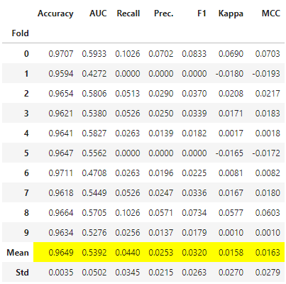
Let’s take a look at the parameters that were used during the training.
print(rf)
RandomForestClassifier(bootstrap=True, ccp_alpha=0.0, class_weight='balanced',
                       criterion='gini', max_depth=None, max_features='auto',
                       max_leaf_nodes=None, max_samples=None,
                       min_impurity_decrease=0.0, min_impurity_split=None,
                       min_samples_leaf=1, min_samples_split=2,
                       min_weight_fraction_leaf=0.0, n_estimators=100,
                       n_jobs=-1, oob_score=False, random_state=22, verbose=0,
                       warm_start=False)
Optimization
Let’s make some hyperparameter tunning to the model to attempt to optimize it.
The tune_model function automatically tunes the hyperparameters of a model using Random Grid Search on a pre-defined search space. It outputs a new scoring grid with cross-validated scores by fold (default is 10 folds) that shows Accuracy, AUC, Recall, Precision, F1, Kappa, and MCC by fold for the best tunned model.
To use the custom search grid with the parameters ranges, the custom_grid parameter can be passed in the tune_model function.
The hyperparameters do not work alone (univariate) but in conjunction with each other (multivariate). Understanding the impact of hyperparameters on the model’s performance becomes even more important when deciding the search space for a grid search. Choosing the wrong search space can lead to wasted wall clock time while not improving the model performance. The pycaret package helps us a lot at this point, as it saves a lot of automation time.
Gridsearch does an exhaustive search over specified parameter values for an estimator. Grid Search uses a different combination of all the specified hyperparameters and their values and calculates the performance for each combination and selects the best value for the hyperparameters. This can make the processing time-consuming and expensive based on the number of hyperparameters involved.
When tunning hyperparameters it’s a challenge to decide which ones to tune.
Tunning the max_depth parameter will manage how deep the tree can grow down. The depth of the trees are proportional to the model complexity because it will have more splits and learn more details about the data. This seems like a good thing, to learn details from the data, but it can actually be a curse once it's the root of the overfitting problem (when the model fits so well to the data that it loses the ability to generalize on unseen data).
The min_samples_split and min_samples_leaf can also help control overfitting as they ensure that more than one samples will be responsible for every decision in the tree. They control the amount of elements needed before splitting so the models doesn't create lots of branches exclusively for one sample each. It let's the leaves have some impurity other than zero. A very small number can lead to overfitting whereas a large one will keep the tree from learning important details of the data. In this case where we have the imbalanced class issue, adopting a small number can be a good strategy because the zones where the minority class will be in majority are likely to be very small, so setting a low number can help with that.
Let’s experiment with some values for those and watch for performance improvement.
# define search space
params = {"max_depth": [5, 8, 11],
          "min_samples_split": [3, 5, 7],
          "min_samples_leaf": [4, 7, 10]}# tune model
t_rf = tune_model(rf, optimize = 'AUC',
                  custom_grid = params)
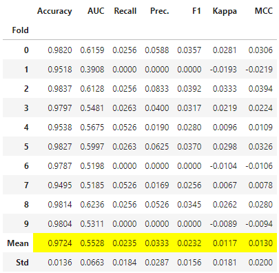
print(t_rf)RandomForestClassifier(bootstrap=True, ccp_alpha=0.0, class_weight='balanced',
                       criterion='gini', max_depth=8, max_features='auto',
                       max_leaf_nodes=None, max_samples=None,
                       min_impurity_decrease=0.0, min_impurity_split=None,
                       min_samples_leaf=10, min_samples_split=7,
                       min_weight_fraction_leaf=0.0, n_estimators=100,
                       n_jobs=-1, oob_score=False, random_state=22, verbose=0,
                       warm_start=False)
Evaluating model
Let’s make some plots so we can better understand the model performance.
# plot auc
plot_model(t_rf, plot = 'auc')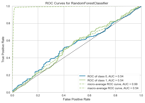
# plot confusion matrix
plot_model(t_rf, plot = 'confusion_matrix',
           plot_kwargs = {'percent' : True})
Because the target variable is highly imbalanced, even though we addressed it with the SMOTE method before training the model, it still isn't exactly "real data" so it's hard to have the model behave well under this circumstance.
The accuracy is high for the majority class (99%) and very low for the minority class (0%), this is caused by a lack of representation of the minority class.
The issue we face here is exactly that we have too many FN — False Negatives (ositive predicted wrongly as negative) which means that for individuals who actually responded to the campaing, our model predicted that they wouldn’t respond.
That would make us miss the chance of acquiring that customer because he wouln’t be on the marketing target (wrongly).
Improvement
Hyperparameter tunning can improve a model’s performance because it’s a refinement. It should be done as an “icing on the cake” refinement when the model has already reached a satisfactory performance.
In this case, the model’s performance isn’t satisfactory so the hyperparameter tunning has little effect on the overall performance.
Highly imbalanced datasets are very challenging to make predictions on. So we should be proud for getting this far up the task!
As a business perspective, my recommendation for improvement of the model is to collect more datapoints so the disparity can be lowered and model can perform better.
Make predictions
Now it’s time to make predictions on the test dataset!!
We won’t be able to evaluate our predictions because the test dataset doesn’t have the target column.
Let’s do it!
# make predicted dataset
df_predicted = predict_model(rf, data = df_test)
df_predicted.head()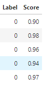
There we go, we’ve made predictions on the test dataset! Two new columns we added to the dataframe are Label (the prediction) and Score (the probability of the prediction).
Let’s check how the label variable is distributed on the predicted dataset.
0    41940
1      893
Name: Label, dtype: int64


Response = 2.13 %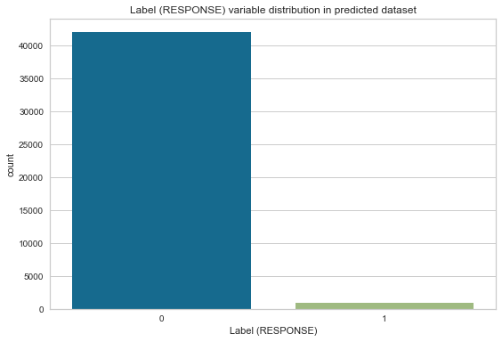
It’s coherent with the training data distribution.
Thank you for your time!
Thanks for following all the way here! This was a very cool project to work on.
Let me know if you have any questions or feedbacks, I’d love to hear from you!
You can find the full code for this project here and you can get in touch with me here.
Special thanks to Arvato Financial Solutions for providing the data and to Udacity for proposing this Capstone Project at the Data Science Nanodegree Program.